S&P 500 Volatility Clusters

Author

Jianyuan(Andy) Hu

Published

December 17, 2024

Project

Goal: Use the broad stock index to model and understand the index volatility levels.

Key methodology: Use KMeans to build clustering model and then volatility regimes and then build transitional probability distribution among the regimes

Import Library

Code

import pyprojroot
from pyprojroot.here import here
import os

import yfinance as yf
import pandas as pd
import numpy as np
import ibis
import ibis.selectors as s
from ibis import _
ibis.options.interactive = True
ibis.options.repr.interactive.max_rows = 20

from plotnine import ggplot, geom_line, geom_path, aes, facet_wrap, labs, scale_x_continuous, theme, element_text, scale_y_continuous, scale_x_date, scale_color_manual
import matplotlib.pyplot as plt
from sklearn.cluster import KMeans
from sklearn.preprocessing import MinMaxScaler

Project File Paths

Code

base_path = pyprojroot.find_root(pyprojroot.has_file('.here'))
output_dir = os.path.join(base_path, "Data", "out")

Import Data

Get a list of S&P 500 price index daily

Code

# Define the ticker symbol for the S&P 500 index
ticker = '^GSPC'

# Define the start and end dates
start_date = '2013-01-01'
end_date = '2024-12-26'

# Fetch the historical data
sp500_data = yf.download(ticker, start=start_date, end=end_date, multi_level_index=False).reset_index()

# Display the data
sp500_data.head(10)

	Date	Close	High	Low	Open	Volume
0	2013-01-02	1462.420044	1462.430054	1426.189941	1426.189941	4202600000
1	2013-01-03	1459.369995	1465.469971	1455.530029	1462.420044	3829730000
2	2013-01-04	1466.469971	1467.939941	1458.989990	1459.369995	3424290000
3	2013-01-07	1461.890015	1466.469971	1456.619995	1466.469971	3304970000
4	2013-01-08	1457.150024	1461.890015	1451.640015	1461.890015	3601600000
5	2013-01-09	1461.020020	1464.729980	1457.150024	1457.150024	3674390000
6	2013-01-10	1472.119995	1472.300049	1461.020020	1461.020020	4081840000
7	2013-01-11	1472.050049	1472.750000	1467.579956	1472.119995	3340650000
8	2013-01-14	1470.680054	1472.050049	1465.689941	1472.050049	3003010000
9	2013-01-15	1472.339966	1473.310059	1463.760010	1470.670044	3135350000

Clean data with ibis framework. We only need to keep Date and Close columns. Since data is downloaded live, we also archive a copy of data.

It is totally okay to use Pandas to clean the data. It’s just a personal preference that I prefer the modernized and portable syntax of ibis framework.

Code

# import to duckdb backend of ibis framework
sp500_data_ibis = ibis.memtable(data=sp500_data)

sp500_data_cleaned = (
    sp500_data_ibis.select("Date", "Close")
        .mutate(Date = _.Date.date(), Close = _.Close.round(digits = 2))
)
# export a csv copy
sp500_data_cleaned.to_csv(path = os.path.join(output_dir, "sp500_close.csv")) 

# preview of data
sp500_data_cleaned

┏━━━━━━━━━━━━┳━━━━━━━━━┓
┃ Date       ┃ Close   ┃
┡━━━━━━━━━━━━╇━━━━━━━━━┩
│ date       │ float64 │
├────────────┼─────────┤
│ 2013-01-02 │ 1462.42 │
│ 2013-01-03 │ 1459.37 │
│ 2013-01-04 │ 1466.47 │
│ 2013-01-07 │ 1461.89 │
│ 2013-01-08 │ 1457.15 │
│ 2013-01-09 │ 1461.02 │
│ 2013-01-10 │ 1472.12 │
│ 2013-01-11 │ 1472.05 │
│ 2013-01-14 │ 1470.68 │
│ 2013-01-15 │ 1472.34 │
│ 2013-01-16 │ 1472.63 │
│ 2013-01-17 │ 1480.94 │
│ 2013-01-18 │ 1485.98 │
│ 2013-01-22 │ 1492.56 │
│ 2013-01-23 │ 1494.81 │
│ 2013-01-24 │ 1494.82 │
│ 2013-01-25 │ 1502.96 │
│ 2013-01-28 │ 1500.18 │
│ 2013-01-29 │ 1507.84 │
│ 2013-01-30 │ 1501.96 │
│ …          │       … │
└────────────┴─────────┘

Calculate Moving Average and Volatility

Code

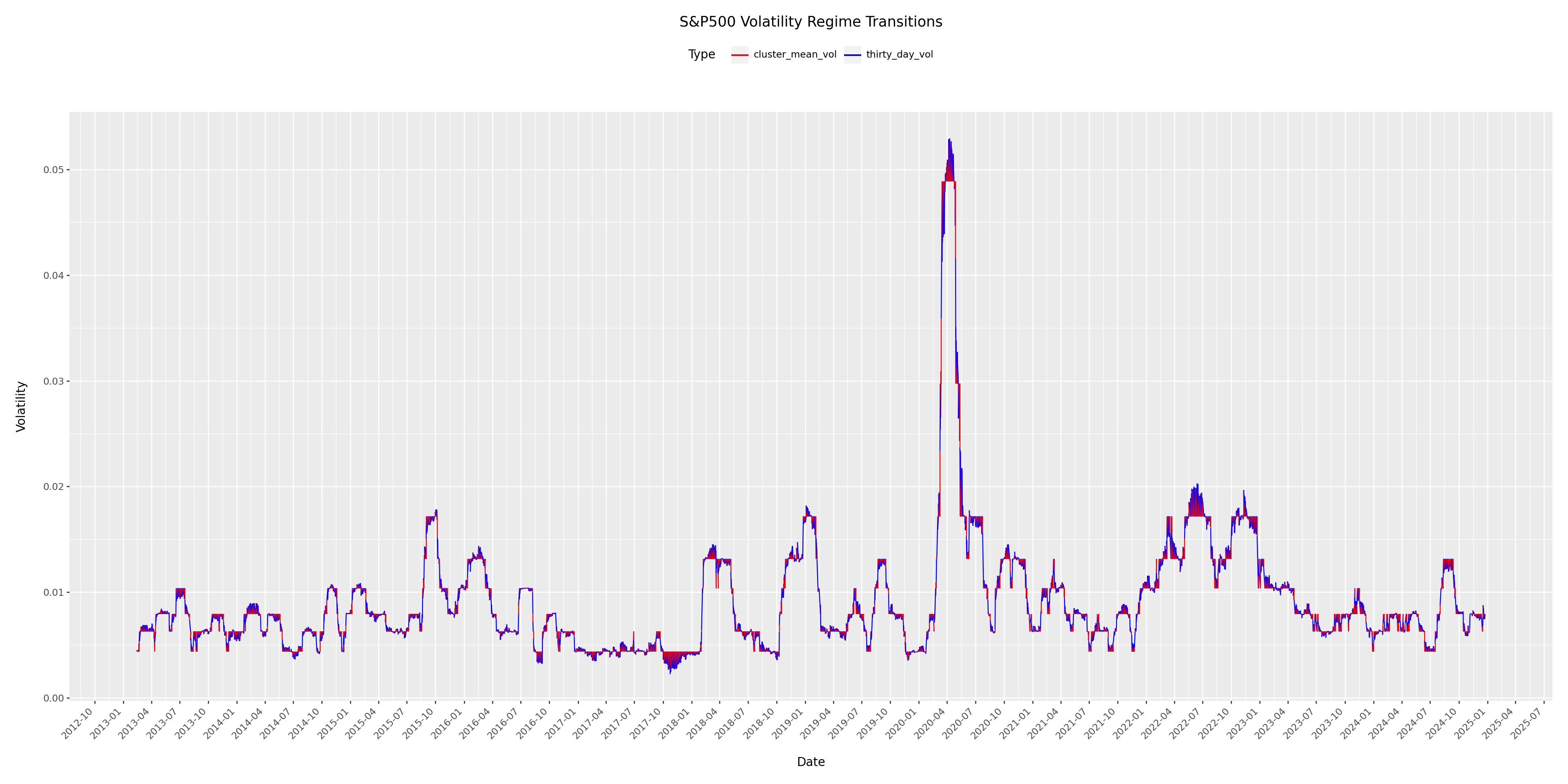
return_window = ibis.window(preceding=30, following=0, order_by="Date")

sp500_data_transformed = (sp500_data_cleaned.mutate(Previous_Close = _.Close.lag())
    .mutate(Daily_Return = ((_.Close - _.Previous_Close)/_.Previous_Close).round(digits = 6))
    .mutate(thirty_day_vol = ibis.ifelse(
        _.Daily_Return.count().over(return_window) >= 30, 
        _.Daily_Return.std().over(return_window).round(digits = 6), 
        None))
)

sp500_vol_no_null = sp500_data_transformed.filter(_.thirty_day_vol != None)
sp500_vol_dates = sp500_vol_no_null.select("Date").mutate(index = ibis.row_number())
sp500_vol = sp500_vol_no_null.select("thirty_day_vol")

# bring to pandas dataframes to be more compatible with sklearn APIs
sp500_vol_pd = sp500_vol.to_pandas()

Train KMeans Model

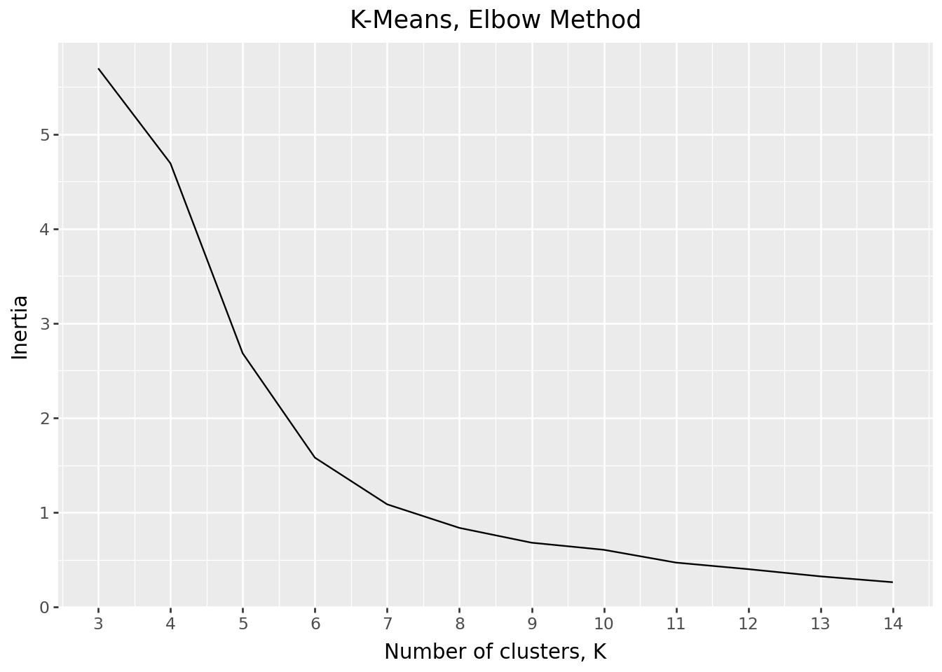
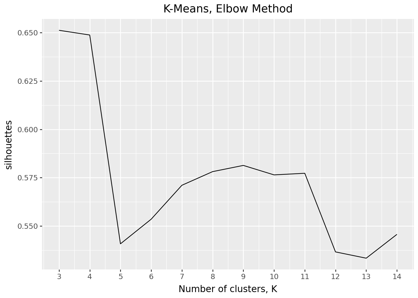
Find the Optimal K, using elbow method

In the following “elbow charts”, trade off between inertia and silhouette scores, we settle at 9 clusters, as it gives a relatively high silhouette scores whil keeping a relatively low inertia.

Code

def find_best_k_for_kmeans_clustering(dataframe, scaler, kmin, kmax,  random_state=42, figheight=8, figwidth=10):
    scalermethod = scaler;
    dataframe_scaled = pd.DataFrame(data=scaler.fit_transform(dataframe[dataframe.columns]), columns=dataframe.columns);
    from sklearn.metrics import silhouette_score, silhouette_samples;
    inertias = {}
    silhouettes = {}
    for k in range(kmin, kmax):
        kmeans = KMeans(n_clusters=k, random_state=random_state).fit(dataframe_scaled)
        inertias[k] = kmeans.inertia_
        silhouettes[k] = silhouette_score(dataframe_scaled, kmeans.labels_, metric='euclidean')
    inertias_df = ibis.memtable(list(inertias.items()), columns=["cluster", "inertia"])
    silhouettes_df = ibis.memtable(list(silhouettes.items()), columns=["cluster", "silhouettes"])
    metrics_df = inertias_df.left_join(silhouettes_df, "cluster").select(~s.contains("_right"))
    return metrics_df

kmeans_metrics_df = find_best_k_for_kmeans_clustering(sp500_vol_pd, scaler=MinMaxScaler(), kmin=3, kmax=15)

kmeans_metrics_df

┏━━━━━━━━━┳━━━━━━━━━━┳━━━━━━━━━━━━━┓
┃ cluster ┃ inertia  ┃ silhouettes ┃
┡━━━━━━━━━╇━━━━━━━━━━╇━━━━━━━━━━━━━┩
│ int64   │ float64  │ float64     │
├─────────┼──────────┼─────────────┤
│       3 │ 5.694822 │    0.651185 │
│       4 │ 4.690729 │    0.648749 │
│       5 │ 2.682729 │    0.540790 │
│       6 │ 1.579715 │    0.553520 │
│       7 │ 1.086568 │    0.571062 │
│       8 │ 0.837567 │    0.578115 │
│       9 │ 0.681040 │    0.581327 │
│      10 │ 0.605977 │    0.576432 │
│      11 │ 0.470595 │    0.577266 │
│      12 │ 0.401481 │    0.536613 │
│      13 │ 0.325140 │    0.533363 │
│      14 │ 0.263371 │    0.545676 │
└─────────┴──────────┴─────────────┘

Create “elbow chart” for inertia (sum of squared distances within each cluster).

We are looking for the number of clusters that yield the relatively lower “turning” of the line.

Code

(
    ggplot(kmeans_metrics_df, aes("cluster", "inertia"))
    + geom_line()
    + scale_x_continuous(breaks=range(3,15))
    + labs(
        x="Number of clusters, K",
        y="Inertia",
        title="K-Means, Elbow Method")
)

Create “elbow chart” for silhouette scores (measuring separation among clusters).

We are looking for the number of clusters that yield the relatively higher “turning” of the line.

Code

(
    ggplot()
    + geom_line(kmeans_metrics_df, aes("cluster", "silhouettes"))
    + scale_x_continuous(breaks=range(3,15))
    + labs(
        x="Number of clusters, K",
        y="silhouettes",
        title="K-Means, Elbow Method")
)

Based on the outputs and criteria, it seems 8 clusters are appropriate.

Train the Optimal KMeans Model and Cluster Volatility

Train the optimal KMeans model and predict the cluster label and then cluster volatilities into 9 different clusters.

Code

def predict_cluster_with_kmeans(dataframe, optimal_k, scaler, Random_State=42):
    from sklearn.cluster import KMeans;
    kmeans = KMeans(n_clusters=optimal_k, random_state=Random_State);
    dataframe_scaled = pd.DataFrame(data=scaler.fit_transform(dataframe[dataframe.columns]), columns=dataframe.columns);
    dataframe['cluster'] = kmeans.fit_predict(dataframe_scaled)
    return dataframe

sp500_vol_pred = predict_cluster_with_kmeans(dataframe=sp500_vol_pd, optimal_k=8, scaler=MinMaxScaler())

sp500_vol_pred.head(10)

	thirty_day_vol	cluster
0	0.004513	0
1	0.004457	0
2	0.004543	0
3	0.005142	0
4	0.005258	0
5	0.005384	6
6	0.006422	6
7	0.006374	6
8	0.006736	6
9	0.006735	6

View the descriptive stats on each cluster.

Code

sp500_vol_pred = (
    ibis.memtable(data=sp500_vol_pred)
    # adding the dates back to the volatility dataset
        .mutate(index = ibis.row_number())
        .left_join(sp500_vol_dates, "index")
        .select(~s.startswith("index"))
)

(
    sp500_vol_pred.aggregate(
            by = "cluster",
            count = _.thirty_day_vol.count(), 
            mean = _.thirty_day_vol.mean(),
            max =  _.thirty_day_vol.max(),
            median = _.thirty_day_vol.median(), 
            min = _.thirty_day_vol.min())
        .order_by(_.cluster)
)

┏━━━━━━━━━┳━━━━━━━┳━━━━━━━━━━┳━━━━━━━━━━┳━━━━━━━━━━┳━━━━━━━━━━┓
┃ cluster ┃ count ┃ mean     ┃ max      ┃ median   ┃ min      ┃
┡━━━━━━━━━╇━━━━━━━╇━━━━━━━━━━╇━━━━━━━━━━╇━━━━━━━━━━╇━━━━━━━━━━┩
│ int32   │ int64 │ float64  │ float64  │ float64  │ float64  │
├─────────┼───────┼──────────┼──────────┼──────────┼──────────┤
│       0 │   517 │ 0.004371 │ 0.005327 │ 0.004471 │ 0.002251 │
│       1 │   349 │ 0.013144 │ 0.015148 │ 0.013046 │ 0.011789 │
│       2 │    31 │ 0.048867 │ 0.052927 │ 0.050229 │ 0.041277 │
│       3 │   704 │ 0.007931 │ 0.009160 │ 0.007856 │ 0.007118 │
│       4 │    14 │ 0.029730 │ 0.035864 │ 0.030857 │ 0.023744 │
│       5 │   229 │ 0.017168 │ 0.023409 │ 0.016761 │ 0.015194 │
│       6 │   732 │ 0.006277 │ 0.007115 │ 0.006308 │ 0.005332 │
│       7 │   410 │ 0.010369 │ 0.011763 │ 0.010353 │ 0.009173 │
└─────────┴───────┴──────────┴──────────┴──────────┴──────────┘

Create the bridging table to relabel clusters.

Relabel the cluster in ascending order of mean volatility of each regime

This is used to create the transitional probability table later.

Code

sp500_vol_pred_cluster_bridge = (
    sp500_vol_pred.aggregate(
        by = _.cluster, 
        cluster_mean_vol = _.thirty_day_vol.mean())
        .order_by(_.cluster_mean_vol)
        .mutate(cluster_new = ibis.row_number())
)

sp500_vol_pred_relabelled = (
    sp500_vol_pred.left_join(sp500_vol_pred_cluster_bridge, _.cluster == sp500_vol_pred_cluster_bridge.cluster)
        .drop(["cluster", "cluster_right"])
        .rename(cluster = "cluster_new")
)

sp500_vol_pred_relabelled

┏━━━━━━━━━━━━━━━━┳━━━━━━━━━━━━┳━━━━━━━━━━━━━━━━━━┳━━━━━━━━━┓
┃ thirty_day_vol ┃ Date       ┃ cluster_mean_vol ┃ cluster ┃
┡━━━━━━━━━━━━━━━━╇━━━━━━━━━━━━╇━━━━━━━━━━━━━━━━━━╇━━━━━━━━━┩
│ float64        │ date       │ float64          │ int64   │
├────────────────┼────────────┼──────────────────┼─────────┤
│       0.004513 │ 2013-02-14 │         0.004371 │       0 │
│       0.004457 │ 2013-02-15 │         0.004371 │       0 │
│       0.004543 │ 2013-02-19 │         0.004371 │       0 │
│       0.005142 │ 2013-02-20 │         0.004371 │       0 │
│       0.005258 │ 2013-02-21 │         0.004371 │       0 │
│       0.005384 │ 2013-02-22 │         0.006277 │       1 │
│       0.006422 │ 2013-02-25 │         0.006277 │       1 │
│       0.006374 │ 2013-02-26 │         0.006277 │       1 │
│       0.006736 │ 2013-02-27 │         0.006277 │       1 │
│       0.006735 │ 2013-02-28 │         0.006277 │       1 │
│       0.006740 │ 2013-03-01 │         0.006277 │       1 │
│       0.006768 │ 2013-03-04 │         0.006277 │       1 │
│       0.006891 │ 2013-03-05 │         0.006277 │       1 │
│       0.006879 │ 2013-03-06 │         0.006277 │       1 │
│       0.006855 │ 2013-03-07 │         0.006277 │       1 │
│       0.006881 │ 2013-03-08 │         0.006277 │       1 │
│       0.006887 │ 2013-03-11 │         0.006277 │       1 │
│       0.006874 │ 2013-03-12 │         0.006277 │       1 │
│       0.006853 │ 2013-03-13 │         0.006277 │       1 │
│       0.006894 │ 2013-03-18 │         0.006277 │       1 │
│              … │ …          │                … │       … │
└────────────────┴────────────┴──────────────────┴─────────┘

Review the key volatility stats based on final clusters:

Code

sp500_vol_pred_relabelled_summary = (
    sp500_vol_pred_relabelled.aggregate(
            by = "cluster",
            count = _.thirty_day_vol.count(), 
            mean = _.thirty_day_vol.mean(),
            max =  _.thirty_day_vol.max(),
            median = _.thirty_day_vol.median(), 
            min = _.thirty_day_vol.min())
        .order_by(_.cluster)
)

sp500_vol_pred_relabelled_summary

┏━━━━━━━━━┳━━━━━━━┳━━━━━━━━━━┳━━━━━━━━━━┳━━━━━━━━━━┳━━━━━━━━━━┓
┃ cluster ┃ count ┃ mean     ┃ max      ┃ median   ┃ min      ┃
┡━━━━━━━━━╇━━━━━━━╇━━━━━━━━━━╇━━━━━━━━━━╇━━━━━━━━━━╇━━━━━━━━━━┩
│ int64   │ int64 │ float64  │ float64  │ float64  │ float64  │
├─────────┼───────┼──────────┼──────────┼──────────┼──────────┤
│       0 │   517 │ 0.004371 │ 0.005327 │ 0.004471 │ 0.002251 │
│       1 │   732 │ 0.006277 │ 0.007115 │ 0.006308 │ 0.005332 │
│       2 │   704 │ 0.007931 │ 0.009160 │ 0.007856 │ 0.007118 │
│       3 │   410 │ 0.010369 │ 0.011763 │ 0.010353 │ 0.009173 │
│       4 │   349 │ 0.013144 │ 0.015148 │ 0.013046 │ 0.011789 │
│       5 │   229 │ 0.017168 │ 0.023409 │ 0.016761 │ 0.015194 │
│       6 │    14 │ 0.029730 │ 0.035864 │ 0.030857 │ 0.023744 │
│       7 │    31 │ 0.048867 │ 0.052927 │ 0.050229 │ 0.041277 │
└─────────┴───────┴──────────┴──────────┴──────────┴──────────┘

Plot the Regime vs Actual thirty_day_Vol

In the following graph, you can see how actual 30-day volatility compares to (shaded in red) their major volatility cluster.

Code

sp500_vol_pred_pivoted = (
    sp500_vol_pred_relabelled.pivot_longer(col=["thirty_day_vol", "cluster_mean_vol"], names_to="Type", values_to="Volatility")
    .order_by(_.Type, _.Date)
)

(
    ggplot(sp500_vol_pred_pivoted, aes(x = "Date"))
    + geom_line(aes(y = "Volatility", color = "Type", group = 1), stat = "identity")
    + scale_color_manual(values=dict(thirty_day_vol = "blue", cluster_mean_vol = "red"))
    + scale_x_date(date_breaks="3 month", date_labels="%Y-%m")
    + labs(
        x = "Date", 
        y = "Volatility",
        title="S&P500 Volatility Regime Transitions" )
    + theme( 
        figure_size=(20, 10),
        legend_position='top',
        axis_text_x=element_text(rotation=45, hjust=1) )
)

Calculate Transition Probability

create cluster transitions counts dataframe

Code

sp500_vol_pred_shifted = (
    sp500_vol_pred.select(cluster_from = "cluster")
        .mutate(
            cluster_from = _.cluster_from.cast("String"),
            cluster_to = _.cluster_from.lead(1).cast("String"))
        # remove NAs from lead()
        .filter(_.cluster_to != None)
)
sp500_vol_pred_shifted

┏━━━━━━━━━━━━━━┳━━━━━━━━━━━━┓
┃ cluster_from ┃ cluster_to ┃
┡━━━━━━━━━━━━━━╇━━━━━━━━━━━━┩
│ string       │ string     │
├──────────────┼────────────┤
│ 0            │ 0          │
│ 0            │ 0          │
│ 0            │ 0          │
│ 0            │ 0          │
│ 0            │ 6          │
│ 6            │ 6          │
│ 6            │ 6          │
│ 6            │ 6          │
│ 6            │ 6          │
│ 6            │ 6          │
│ 6            │ 6          │
│ 6            │ 6          │
│ 6            │ 6          │
│ 6            │ 6          │
│ 6            │ 6          │
│ 6            │ 6          │
│ 6            │ 6          │
│ 6            │ 6          │
│ 6            │ 6          │
│ 6            │ 6          │
│ …            │ …          │
└──────────────┴────────────┘

Code

# get a frequecy of each cluster to calculate relative frequency of each transition type, see below
sp500_cluster_vol_count = (
    sp500_vol_pred.aggregate(
                by = "cluster",
                count = _.thirty_day_vol.count())
    .mutate(cluster = _.cluster.cast("String"))
)

vol_transition_table = (
        # perform crosstabbing between cluster_from and cluster_to to understand count of transitions 
    sp500_vol_pred_shifted
        .mutate(counter = 1)
        .pivot_wider(names_from ="cluster_to", values_from="counter", values_agg="sum", values_fill=0, names_sort=True)
        # add cluster frequency
        .left_join(
            right = sp500_cluster_vol_count, 
            predicates= _.cluster_from == sp500_cluster_vol_count.cluster
        )
        # clean up data
        .drop(_.cluster_from)
        .order_by(_.cluster)
        .relocate(_.cluster, before="0")
)
vol_transition_table

┏━━━━━━━━━┳━━━━━━━┳━━━━━━━┳━━━━━━━┳━━━━━━━┳━━━━━━━┳━━━━━━━┳━━━━━━━┳━━━━━━━┳━━━━━━━┓
┃ cluster ┃ 0     ┃ 1     ┃ 2     ┃ 3     ┃ 4     ┃ 5     ┃ 6     ┃ 7     ┃ count ┃
┡━━━━━━━━━╇━━━━━━━╇━━━━━━━╇━━━━━━━╇━━━━━━━╇━━━━━━━╇━━━━━━━╇━━━━━━━╇━━━━━━━╇━━━━━━━┩
│ string  │ int64 │ int64 │ int64 │ int64 │ int64 │ int64 │ int64 │ int64 │ int64 │
├─────────┼───────┼───────┼───────┼───────┼───────┼───────┼───────┼───────┼───────┤
│ 0       │   466 │     5 │     0 │     8 │     0 │     2 │    32 │     4 │   517 │
│ 1       │     2 │   300 │     0 │     4 │     0 │    15 │     5 │    23 │   349 │
│ 2       │     0 │     0 │    29 │     0 │     1 │     1 │     0 │     0 │    31 │
│ 3       │    11 │     5 │     0 │   586 │     1 │     1 │    73 │    26 │   704 │
│ 4       │     0 │     0 │     1 │     0 │    11 │     1 │     0 │     1 │    14 │
│ 5       │     0 │    14 │     1 │     4 │     1 │   203 │     1 │     5 │   229 │
│ 6       │    35 │     1 │     0 │    70 │     0 │     3 │   614 │     9 │   732 │
│ 7       │     2 │    24 │     0 │    32 │     0 │     3 │     7 │   342 │   410 │
└─────────┴───────┴───────┴───────┴───────┴───────┴───────┴───────┴───────┴───────┘

Code

# calculate relative frequencies
vol_transition_freq_table = vol_transition_table.mutate(s.across(s.numeric(), func = _ / vol_transition_table['count'])).drop("count")

vol_transition_freq_table

┏━━━━━━━━━┳━━━━━━━━━━┳━━━━━━━━━━┳━━━━━━━━━━┳━━━━━━━━━━┳━━━━━━━━━━┳━━━━━━━━━━┳━━━━━━━━━━┳━━━━━━━━━━┓
┃ cluster ┃ 0        ┃ 1        ┃ 2        ┃ 3        ┃ 4        ┃ 5        ┃ 6        ┃ 7        ┃
┡━━━━━━━━━╇━━━━━━━━━━╇━━━━━━━━━━╇━━━━━━━━━━╇━━━━━━━━━━╇━━━━━━━━━━╇━━━━━━━━━━╇━━━━━━━━━━╇━━━━━━━━━━┩
│ string  │ float64  │ float64  │ float64  │ float64  │ float64  │ float64  │ float64  │ float64  │
├─────────┼──────────┼──────────┼──────────┼──────────┼──────────┼──────────┼──────────┼──────────┤
│ 0       │ 0.901354 │ 0.009671 │ 0.000000 │ 0.015474 │ 0.000000 │ 0.003868 │ 0.061896 │ 0.007737 │
│ 1       │ 0.005731 │ 0.859599 │ 0.000000 │ 0.011461 │ 0.000000 │ 0.042980 │ 0.014327 │ 0.065903 │
│ 2       │ 0.000000 │ 0.000000 │ 0.935484 │ 0.000000 │ 0.032258 │ 0.032258 │ 0.000000 │ 0.000000 │
│ 3       │ 0.015625 │ 0.007102 │ 0.000000 │ 0.832386 │ 0.001420 │ 0.001420 │ 0.103693 │ 0.036932 │
│ 4       │ 0.000000 │ 0.000000 │ 0.071429 │ 0.000000 │ 0.785714 │ 0.071429 │ 0.000000 │ 0.071429 │
│ 5       │ 0.000000 │ 0.061135 │ 0.004367 │ 0.017467 │ 0.004367 │ 0.886463 │ 0.004367 │ 0.021834 │
│ 6       │ 0.047814 │ 0.001366 │ 0.000000 │ 0.095628 │ 0.000000 │ 0.004098 │ 0.838798 │ 0.012295 │
│ 7       │ 0.004878 │ 0.058537 │ 0.000000 │ 0.078049 │ 0.000000 │ 0.007317 │ 0.017073 │ 0.834146 │
└─────────┴──────────┴──────────┴──────────┴──────────┴──────────┴──────────┴──────────┴──────────┘